Naive Bayes Classification in R

The R code for this tutorial can be found on GitHub here: https://github.com/statswithrdotcom/Naive-Bayes-Classification

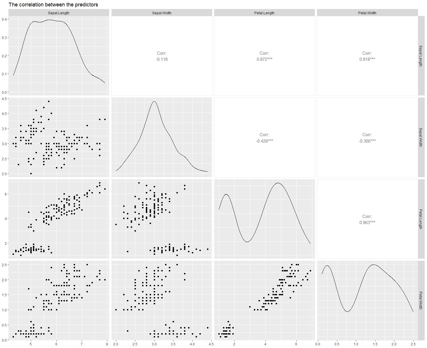
Naive Bayes is a computationally simple, but incredibly effective method for classification. Note that the drawback of this method is that it assumes that your predictor variables are independent, which is almost never true for real data. Luckily, as we will see in the Iris data set this assumption can be obviously false and we still get very good classification accuracy. This model results in a classification accuracy of 97% (for this particular data split), which is higher than the accuracy I found for random forest classification (95%) and neural network-based classification (91%). Although, the neural network-based classification was based on a different split, and I was not focused on obtaining the highest possible accuracy. To start, I am going to go ahead and show the correlation between the predictors, using the ggpairs() function in the “GGally” package, so you can get a visual idea of what I am talking about.

# library GGally for correlation plot
library(GGally)

# load the iris data set
data(iris)

# The correlation plot is made for the predictors
ggpairs(iris[-5], title = "The correlation between the predictors")

Now, we can start with the naive Bayes classification. First, we need to library the “naivebayes” package and split the data into a train and test set. Below this, is the single line of code that creates the naive Bayes model, where the “~.” indicates that we want to use all other variables as predictors.

# library the naive Bayes package
library(naivebayes)

# Choose the Size of training data
Train_N <- 75 # 50% split

# Split the data set into training and test
set.seed(123) #makes it repeatable
Ind <- sample(1:nrow(iris), Train_N, replace = FALSE)
Train <- iris[Ind,]
Test <- iris[-Ind,]

# The naive Bayes model created using the training data
model <- naive_bayes(Species ~ ., data = Train, ntree = Num_Trees)

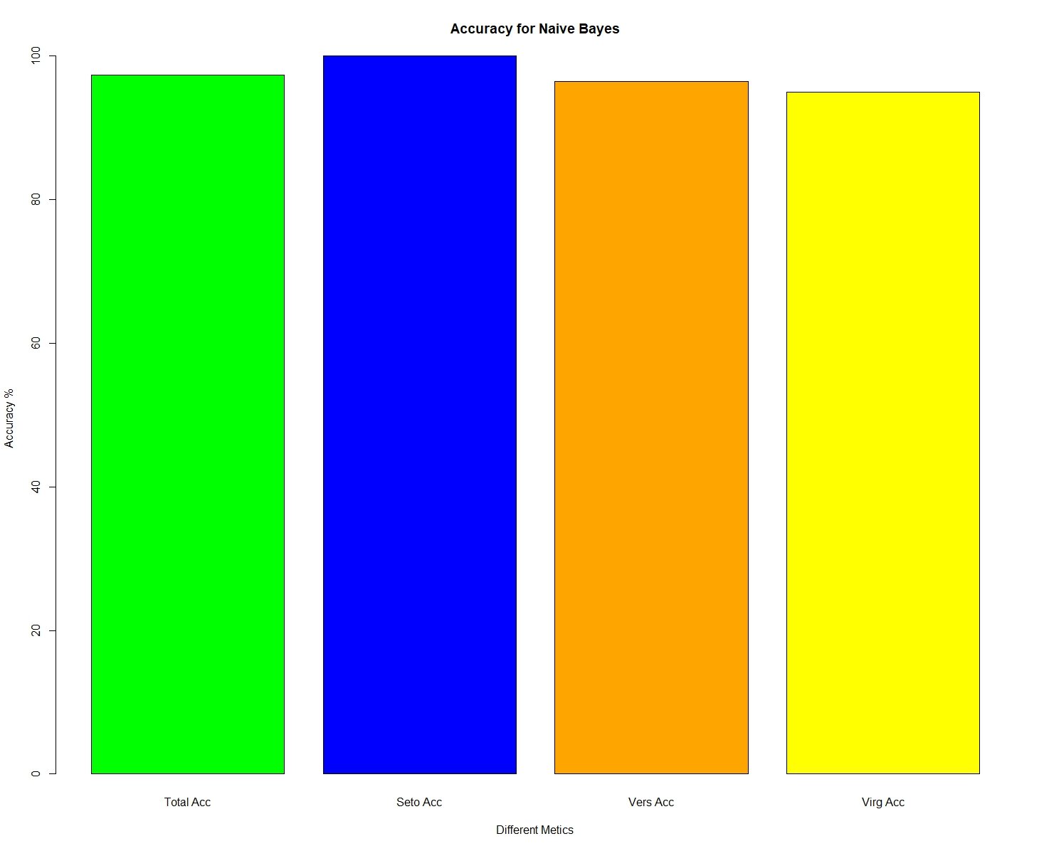
The remainder of the code is nearly identical to the code I used for random forest classification. I am taking the results and tallying the number of correct classifications for each species. Then, I am having R print and produce a bar plot to visually show this. If you want a more detailed explanation, you can refer to the random forest classification tutorial here. Like the random forest model, we see that the setosas are always correctly identified, but the model struggles a bit to distinguish between the versicolor and virginica flowers.

# A data frame containing the predicted and actual flower species
Results <- data.frame(predict(model,Test[,-5]), Test[,5])
names(Results) <- c("Predicted","Actual")

# Initializing values for the loop
Correct <- rep(0,(150-Train_N))
Group_1 <- Group_2 <- Group_3 <- 0
C1 <- C2 <- C3 <- 0

# For loop that iterates through the row indexes of the "Results" data frame
for(i in 1:(150-Train_N)){
# Assigns a 1 to "Correct" if it is correct
if(Results$Predicted[i] == Results$Actual[i]){
Correct[i] = 1
}
# Counts up C1 and accumulates group 1 if correct
if(Results$Actual[i] == "setosa"){
C1 = C1 + 1
if(Correct[i] == 1){Group_1 = Group_1 + 1}
}
# Counts up C2 and accumulates group 2 if correct
if(Results$Actual[i] == "versicolor"){
C2 = C2 + 1
if(Correct[i] == 1){Group_2 = Group_2 + 1}
}
# Counts up C3 and accumulates group 3 if correct
if(Results$Actual[i] == "virginica"){
C3 = C3 + 1
if(Correct[i] == 1){Group_3 = Group_3 + 1}
}
}

# Calculating the percent correct ovar all and by species
Correct_Total = round(sum(Correct)*100/(150-Train_N),2)
Correct_Seto = round(Group_1*100/C1,2)
Correct_Vers = round(Group_2*100/C2,2)
Correct_Virg = round(Group_3*100/C3,2)

# Printing percent correct in the console
print(paste("Total accuracy: ", Correct_Total, "%",
" Setosa accuracy: ", Correct_Seto, "%",
" Versicolor accuracy: ", Correct_Vers, "%",
" Virginica accuracy: ", Correct_Virg, "%", sep = ""))

# Visualizing percent correct as a bar plot
barplot(c(Correct_Total,Correct_Seto,Correct_Vers,Correct_Virg),
names.arg = c("Total Acc","Seto Acc", "Vers Acc", "Virg Acc"),
main = paste("Accuracy for Naive Bayes"),xlab = "Different Metics",
ylab = "Accuracy %", col = c("green","blue","orange","yellow"))